The Ultimate Guide To Learn Excel

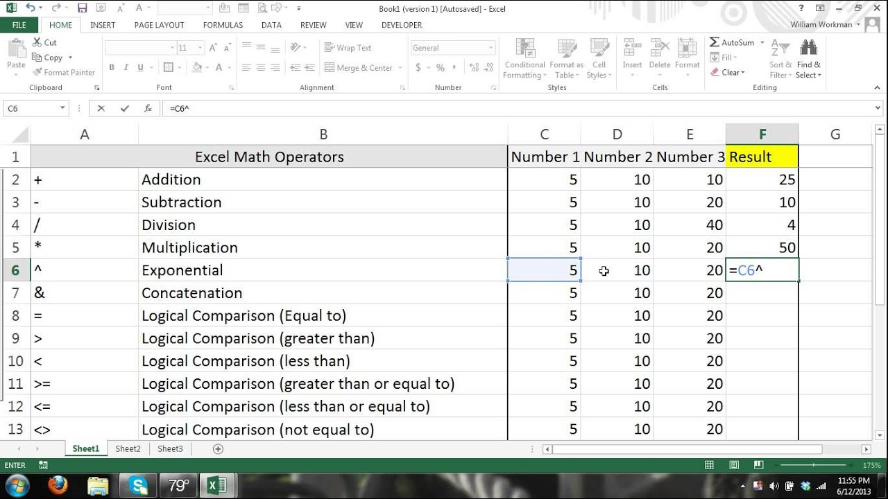
By pushing ctrl+change+center, this will compute as well as return worth from several varieties, instead of just individual cells added to or increased by each other. Computing the amount, item, or ratio of specific cells is easy-- simply use the =AMOUNT formula as well as get in the cells, worths, or series of cells you wish to perform that math on.

If you're seeking to find complete sales earnings from numerous sold devices, for instance, the selection formula in Excel is ideal for you. Here's exactly how you 'd do it: To begin making use of the selection formula, type "=SUM," and in parentheses, enter the first of 2 (or 3, or 4) series of cells you want to multiply together.

This stands for multiplication. Following this asterisk, enter your second variety of cells. You'll be multiplying this second series of cells by the very first. Your development in this formula should currently resemble this: =AMOUNT(C 2: C 5 * D 2:D 5) Ready to press Enter? Not so quickly ... Because this formula is so difficult, Excel reserves a different keyboard command for arrays.

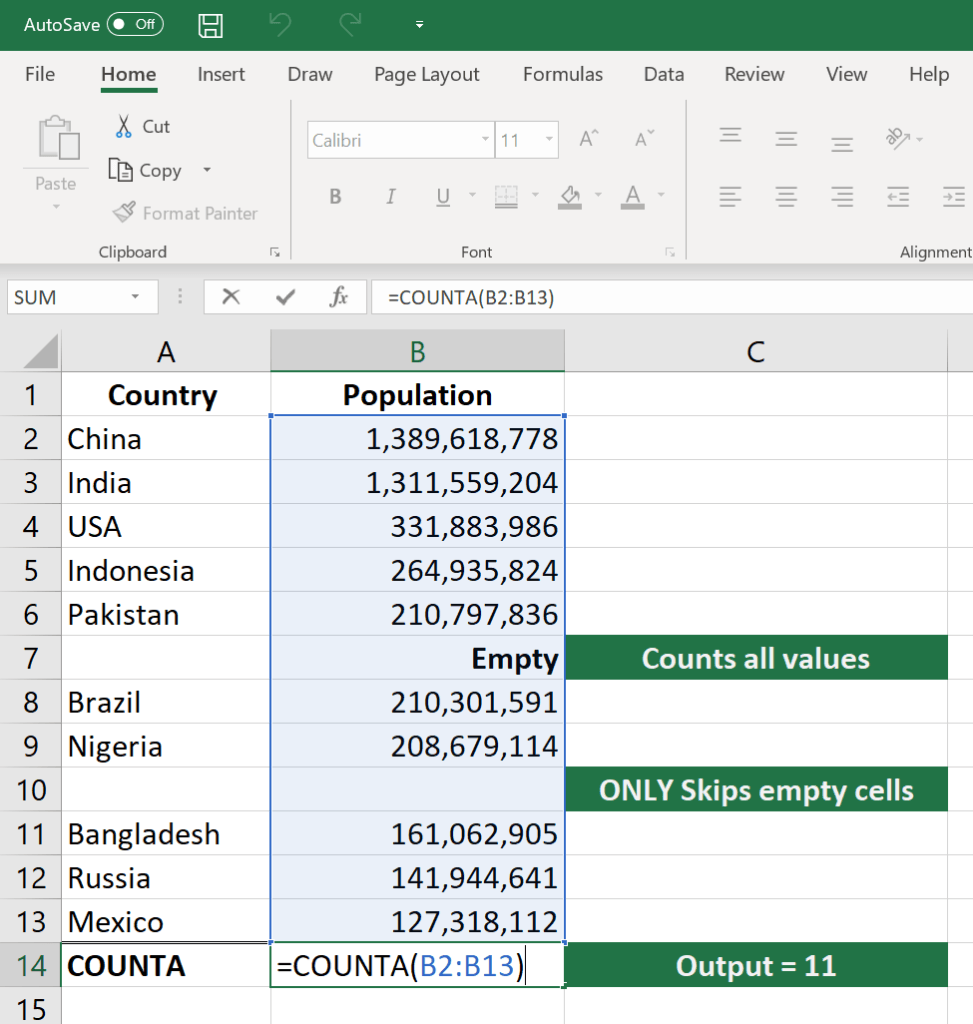
This will recognize your formula as a variety, covering your formula in support characters as well as efficiently returning your item of both varieties integrated. In income estimations, this can minimize your time as well as effort substantially. See the last formula in the screenshot above. The MATTER formula in Excel is signified =COUNT(Begin Cell: End Cell).

As an example, if there are 8 cells with entered worths between A 1 as well as A 10, =MATTER(A 1: A 10) will return a value of 8. The COUNT formula in Excel is especially useful for big spread sheets, in which you desire to see the amount of cells consist of real entries. Don't be deceived: This formula won't do any type of mathematics on the worths of the cells themselves.

Little Known Questions About Sumif Excel.

Utilizing the formula in bold above, you can quickly run a matter of energetic cells in your spread sheet. The outcome will look a little something such as this: To carry out the average formula in Excel, get in the worths, cells, or variety of cells of which you're determining the average in the format, =STANDARD(number 1, number 2, etc.) or =STANDARD(Begin Value: End Value).

Finding the average of a variety of cells in Excel keeps you from needing to discover specific sums and after that doing a different division formula on your total amount. Using =AVERAGE as your initial message entrance, you can allow Excel do all the job for you. For referral, the average of a team of numbers amounts to the sum of those numbers, divided by the variety of products in that team.

This will certainly return the sum of the worths within a wanted range of cells that all meet one requirement. As an example, =SUMIF(C 3: C 12,"> 70,000") would return the sum of worths between cells C 3 as well as C 12 from just the cells that are more than 70,000. Allow's say you wish to figure out the profit you created from a checklist of leads that are connected with details location codes, or compute the sum of particular workers' incomes-- yet only if they drop over a particular quantity.

With the SUMIF function, it does not need to be-- you can easily add up the sum of cells that satisfy particular criteria, like in the salary instance over. The formula: =SUMIF(array, standards, [sum_range] Range: The variety that is being examined utilizing your criteria. Requirements: The requirements that establish which cells in Criteria_range 1 will certainly be totaled [Sum_range]: An optional variety of cells you're mosting likely to accumulate in addition to the first Range got in.

In the example listed below, we intended to compute the amount of the wages that were above $70,000. The SUMIF feature included up the dollar amounts that surpassed that number in the cells C 3 via C 12, with the formula =SUMIF(C 3: C 12,"> 70,000"). The TRIM formula in Excel is denoted =TRIM(text).

Countif Excel Can Be Fun For Everyone

For instance, if A 2 consists of the name" Steve Peterson" with undesirable rooms prior to the very first name, =TRIM(A 2) would return "Steve Peterson" with no rooms in a brand-new cell. Email as well as file sharing are terrific tools in today's work environment. That is, up until among your associates sends you a worksheet with some really cool spacing.

As opposed to meticulously getting rid of and adding areas as needed, you can tidy up any kind of irregular spacing making use of the TRIM function, which is made use of to remove additional rooms from data (other than for single areas in between words). The formula: =TRIM(message). Text: The text or cell from which you want to get rid of spaces.

To do so, we went into =TRIM("A 2") right into the Formula Bar, as well as replicated this for each name below it in a new column next to the column with unwanted areas. Below are a few other Excel solutions you could discover beneficial as your data administration needs expand. Allow's say you have a line of message within a cell that you want to damage down into a couple of various sectors.

Function: Made use of to remove the very first X numbers or personalities in a cell. The formula: =LEFT(text, number_of_characters) Text: The string that you want to remove from. Number_of_characters: The number of personalities that you want to remove beginning from the left-most personality. In the example below, we went into =LEFT(A 2,4) into cell B 2, and also replicated it right into B 3: B 6.

Purpose: Used to remove characters or numbers in the middle based on placement. The formula: =MID(message, start_position, number_of_characters) Text: The string that you want to extract from. Start_position: The placement in the string that you wish to start drawing out from. For instance, the first position in the string is 1.

About Vlookup Excel

In this instance, we entered =MID(A 2,5,2) right into cell B 2, and also duplicated it into B 3: B 6. That permitted us to remove both numbers starting in the 5th placement of the code. Objective: Used to extract the last X numbers or personalities in a cell. The formula: =RIGHT(text, number_of_characters) Text: The string that you desire to draw out from.

formulas of excel sheet formula excel abs excel formulas in tamil